Continuing with the theme of the last post, here I’ll cover support vector machines (SVM) from the ground-up. Relatively speaking, there are many more resources out there on this - most discussions of SVMs do cover the geometry, happily - but nevertheless, it is worth deriving from scratch and comparing to our earlier result.
Again, in classification, we want to find a decision boundary in feature space that separates our classes. Like logistic regression, support vector machines are linear classifiers at their core. We are simply looking for a decision hyperplane.
The question is always: how do we choose the separating hyperplane? Recall from the last post the following example: we have two points in $\mathbb{R}^2$.
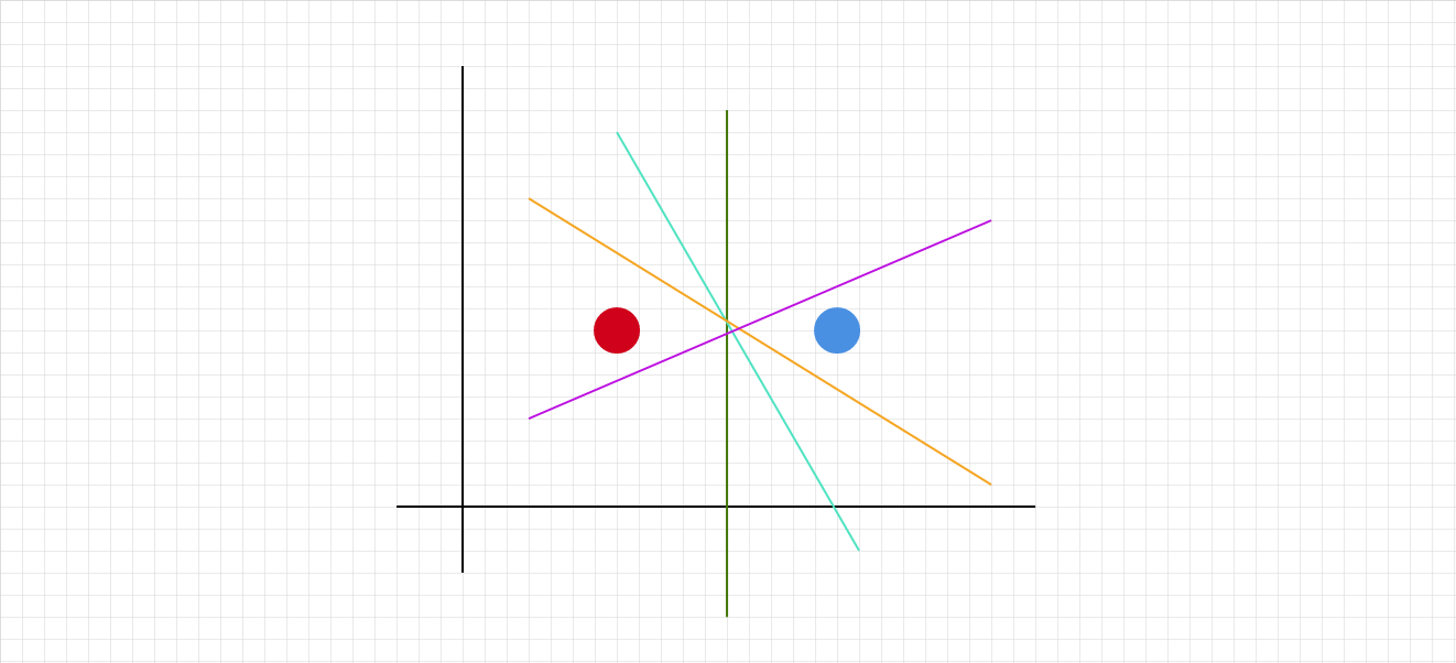
All of these colored lines are separating decision lines! Which one will SVM select?
1. Linearly separable SVM - primal
Let’s begin with the basic linear model:
\[y(x) = w^T\phi(x) + b\]Which defines a hyperplane in feature space. $\phi(x)$ is an arbitrary feature transformation of our training data $x$. It could be the identity transformation, $\phi(x) = x$; it could be a square transformation $\phi(x) = x^2$. More on this here.
We have $N$ input vectors $x_1, …, x_N$ and corresponding target values $t_1, …, t_N$, and $t_n \in \{-1, 1\}$.
Let’s assume that the data is linearly separable in feature space. As we’ve seen previously, we can have multiple candidate decision boundaries. In SVM, we use the idea of the margin - the perpendicular distance between the decision boundary and the closest data point - to decide between them. The SVM’s choice of hyperplane maximizes the margin.
How do we mathematically express the margin? Recall the distance of a point $x$ to the hyperplane $y(x) = w^T\phi(x) + b = 0$ is given by
\[\frac{|y(x)|}{||w||}\]Going back to our assumption of linear separability, we are only interested in solutions where all points are correctly classified - hence $t_ny(x_n) > 0, \forall n$. So the distance of point $x_n$ is:
\[\frac{t_ny(x_n)}{||w||} = \frac{t_n(w^T\phi(x)+b)}{||w||}\]The margin is this distance for the closest point $x_n$, so it is equal to:
\[\frac{1}{||w||}\min_nt_n(w^T\phi(x)+b)\]And the SVM objective to maximize the margin, then, is expressed as:
\[\text{arg max}_{w,b}\frac{1}{||w||}\min_nt_n(w^T\phi(x)+b)\]That is a complex optimization problem! We can turn it into a more tractable form by noticing that we can freely rescale $w^T\phi(x)+b$ without changing the decision boundary. Consider:
\[w^T\phi(x^*)+b = \delta\]Divide both sides to get:
\[\frac{1}{\delta}w^T\phi(x^*) - \frac{b}{\delta} = 1\]But we can just redefine $\hat{w} = \frac{1}{\delta}w$ and $\hat{b} = \frac{b}{\delta}$
\[\hat w^T\phi(x^*)+\hat b = 1\]Which doesn’t change the hyperplane. So we can enforce $t^*(w^T\phi(x^*)+b)=1$ for the closest point to the surface $x^*$.
As a result, all points will satisfy $t_n(w^T\phi(x_n)+b)\geq1, \forall n$.
We the simplify our problem from:
\[\text{arg max}_{w,b}\frac{1}{||w||}\min_nt_n(w^T\phi(x)+b)\]to
\[\text{arg max}_{w,b}\frac{1}{||w||}\] \[\text{subject to }\] \[t_n(w^T\phi(x_n)+b)\geq1, \forall n\]Which is mathematically equivalent to
\[\text{arg min}_{w,b}\frac{1}{2}||w||^2\text{ s.t. }t_n(w^T\phi(x_n)+b)\geq1, \forall n\] \[\text{subject to }\] \[t_n(w^T\phi(x_n)+b)\geq1, \forall n\]This is more mathematically convenient.
2. Dual formulation
To solve this constrained optimization problem, we can use the Lagrangian. Introduce KKT multipliers $a_n \geq 0$ - one for each constraint $t_n(w^T\phi(x_n)+b) \geq 1$. Take note of the signs - as a result we will have to subtract in the Lagrangian.
\[L(w,b,a) = \frac{1}{2}w^Tw - \sum_n a_n(t_n(w^T\phi(x_n)+b)-1)\]If we take the derivatives with respect to $w$ and $b$ we will find:
\[w = \sum_n a_nt_n\phi(x_n)\] \[0 = \sum_n a_nt_n\]And by substituting back into $L(w,b,a)$ we can eliminate $w, b$ to express $L$ completely in terms of $a$:
\[L(a) = \sum_n a_n - \frac{1}{2}\sum_n\sum_m a_na_mt_nt_m\phi(x_n)^T\phi(x_m)\] \[\text{subject to }\] \[a_n \geq 0\] \[\sum_n a_nt_n = 0\]We have the dual representation of the maximum margin problem, where we want to maximize $L(a)$.
Solving from here will yield our optimal $a$ (and thus $w$) and $b$. Going into further detail is beyond my ken, unfortunately.
Predictions for new $x$ can be obtained from:
\[y(x) = w^T\phi(x) + b\] \[y(x) = \sum_n a_nt_n\phi(x_n)^T\phi(x_m) + b\]3. KKT and Complementary slackness
This optimization satisfies the KKT conditions:
\[a_n \geq 0\] \[t_ny(x_n)-1 \geq 0\] \[a_n(t_ny(x_n)-1) = 0\]So it follows that for every point $x_n$, either $a_n=0$ or $t_ny(x_n) = 1$. This complementary slackness property tells us that all points where $a_n=0$ don’t play a role in prediction - they won’t appear in the above sum. The remaining data points are the eponymous support vectors, where $t_ny(x_n)=1$. They lie on the maximum margin hyperplanes.
Practically, this means that after training, most of the training data can be discarded - we only need the support vectors!
This is the reason for the sparsity property of SVM.
4. Comparison to logistic regression
- Logistic regression: we are finding a separating hyperplane that is maximizing the product of the sigmoid-transformed classification margins, over ALL points in the training set: $\prod_i \sigma(y_iw^Tx_i)$. Importantly, logistic regression provides class probabilities for each point $x_i$, which makes sense as the loss function is considering all points.
- SVM: we are finding a separating hyperplane that maximizes the margin, the distance to the closest point. Which is by definition reliant only on the nearest support vectors. Other points can be moved or even removed without affecting the SVM solution! This can be beneficial at test time as after training, we can discard everything but those support vectors. On the other hand, SVM does not provide meaningful class probabilities for each point as a result. The decision boundary is not even considering points that are not the support vectors! So while applying a sigmoid transformation to $w^Tx$ to output a probability makes sense in logistic regression, intuitively it does not in SVM.