Yet Another ML Blog

While trying to make good on my promise of another example of kernels here in the form of kernel density estimation, I thought it made sense to also discuss some simple nonparametric density estimation methods in general.

The general problem we want to solve is density estimation. Given a finite set of observations $x_1, …, x_n$ of a random variable $x$, we wish to estimate its probability density.

1. Parametric vs Nonparametric

A parametric approach to density estimation involves specifying an explicit functional form for the density, controlled by some number of parameters. For instance, we might assume a Gaussian density. Then we are trying to fit our data $x$ to:

\[p(x|\mu, \sigma^2) = \frac{1}{\sqrt{2\pi\sigma^2}}\exp(\frac{-(x-\mu)^2}{2\sigma^2})\]

Meaning that we are trying to find the parameters $\hat{\mu}, \hat{\sigma^2}$ that fit our data $x$ the “best.” Defining “best” and the process of estimating these parameters is a separate topic - we will leave it at this for now. The point is that in a parametric approach we have a functional form and some corresponding small number of parameters (relative to $n$) that we will determine using the dataset.

The number of parameters is a point of emphasis, because parametric approaches are computationally cheaper as a result. The primary limitation is that we have to choose a good functional form. If we choose a density that is a poor model for the true underlying distribution, our performance will always suffer. So parametric approaches are prone to high bias.

Nonparametric approaches do not make such strong assumptions about the form of the distribution. However, the tradeoff is that the number of parameters involved grows with the size of the data $n$. Hence, nonparametric approaches are prone to high variance. This will become clearer in the following examples.

2. Histogram density estimation

Histogram methods are a good simple introduction. Again, we have observations of a continuous random variable $x$ whose density is unknown. To estimate this density with a histogram we simply partition $x$ into distinct bins of width $\Delta_i$ and count the number $n_i$ of observations of $x$ falling in bin $i$. To turn the count into a normalized probability density, we simply divide by $N$ and $\Delta_i$. This is easy to see through geometry - to normalize, we want the area of all the bars to sum to 1. The heights of the bars are $n_i$, the width is $\Delta_i$. So we divide by $N \Delta_i$:

\[p_i = \frac{n_i}{N \Delta_i}\]

Often we will choose the same width for the bins $\Delta$.

Here is an example of histogram density estimation. The data obeys a Gaussian distribution with mean 30 and variance 5. In each successive image the bin width $\Delta$ is increased.

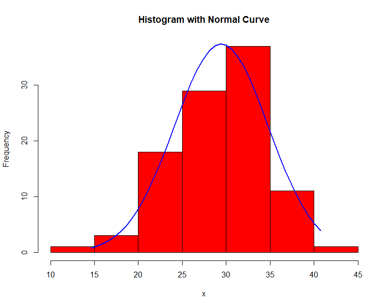
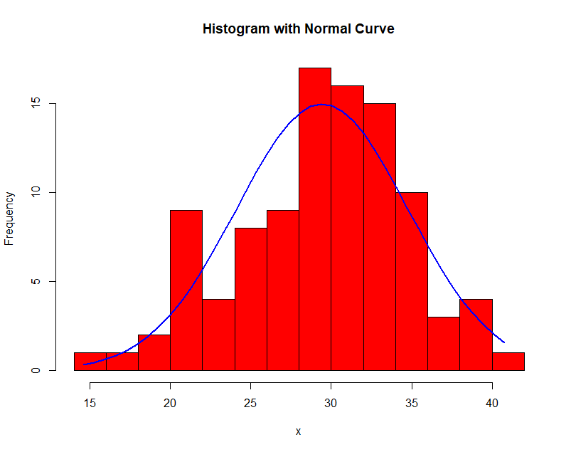
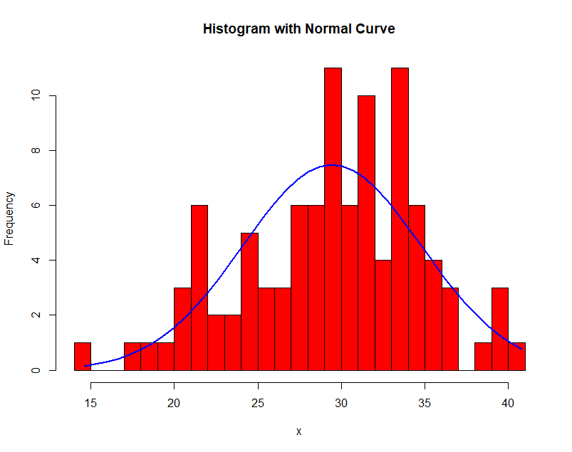
Notice the effect of the choice of $\Delta$! In general, when large, the density is smooth and prone to bias; when small, the density is spiky and prone to overfit.

Histogram density estimation has its advantages. It is easily applied in online learning situations where data points arrive sequentially. We simply have to increment the corresponding bin. Also, once the histogram is computed, we can discard the data set itself, so it is cheap at test time.

But of course, there are drawbacks. First, the bin edges produce artificial discontinuities that aren’t related to the underlying distribution of the data. The second is related to the curse of dimensionality - if we have a $D$ dimensional space and divide it into $M$ bins, we have $M^D$ bins in total! The quantity of data required to provide a meaningful estimate would be extremely large.

3. Beyond histograms

Now lets discuss two of the most common nonparametric estimation methods, kernel density estimators and nearest neighbors. They will handle high dimensionality much more competently. The math involved to reach both models is quite elegant.

We have an unknown density $p(x)$ in $\mathbb{R}^D$. Intuitively, as we’ve seen previously, if we want to estimate the density at a point $x$ it makes sense to consider the local surrounding space. With this in mind, let us define a small region $R$ in $\mathbb{R}^D$ space containing our point $x$. Then the corresponding probability mass $P$ is:

\[P = \int_R p(x)dx\]

We collect $N$ data points from $p(x)$. Every point has some probability, which we define as $P$, of falling in $R$. Let $K$ be the total number of points in $R$. Clearly, it is binomially distributed.

\[Bin(K|N, P) = \frac{N!}{K!(N-K)!}P^K(1-P)^{N-K}\]

Then we know that $E(K) = NP$.

1. Assuming large $N$, we can say $K \approx NP$.
2. Assuming a small $R$ such that $p(x)$ is constant in $R$, we can say $P \approx p(x)V$ where $V$ is the volume of $R$.

These are admittedly contradictory assumptions - but if we are comfortable making them, we arrive at:

\[p(x) = \frac{K}{NV}\]

A beautiful result, but we are not yet done. We don’t have $K$ or $V$! We can only determine one of them with the resources (the data $x$) that we have.

3.1 Kernel density estimation

Suppose we fix $V$ and find $K$ from the data. The simplest example is to assume $R$ as a hypercube centered on $x$. Introducing the Parzen window, a kernel function:

\[k(x, x_i) = \begin{cases} 1, & |x-x_i| \leq \frac{1}{2} \\ 0, & \text{otherwise} \end{cases}\]

The Parzen window mathematically defines our hypercube. Notice that $k(x/h, x_i/h)$ will be $1$ if point $x_i$ lies within a cube of length $h$ centered on $x$, and $0$ otherwise.

Thus the total number of points $K$ that lie in $R$ is:

\[K = \sum_{i=1}^Nk(x/h, x_i/h)\]

Since $R$ is a hypercube of length $h$, the volume is $V=h^D$

So plugging it all back in:

\[p(x) = \frac{1}{Nh^D}\sum_{i=1}^Nk(x/h, x_i/h)\]

Any kernel function can be substituted in; the Parzen window is just a great didactic choice because of its geometric interpretation. Another common choice is a Gaussian kernel, which is of the form:

\[k(x, x_i) = \frac{1}{N}\sum_{i=1}^N \frac{1}{2\pi\sigma^2}^{D/2}\exp{\frac{-||x-x_i||^2}{2\sigma^2}}\]

Recall the idea of a kernel function as measuring similarity between points. Here, when estimating the density at point $x$, the kernel function is weighing points $x_i$ relative to $x$.

In the case of the Parzen window, we are weighing all points within distance $h$ of our center point $x$ at 1 - we are weighing them all the same - and everything else at 0. Then we use those specific points to calculate the density at $x$.

In the case of the Gaussian kernel, we are actually giving some weight to all points $x_i$, but the ones closer to $x$ will receive a higher weight. And the contributions of all these weighted points is combined to estimate the density at $x$.

A spectacular visualization of kernel density estimation can be found here - many thanks, Matthew Conlen!

3.1.1 Drawbacks

Take another look at our final estimate (using Parzen window):

\[p(x) = \frac{1}{Nh^D}\sum_{i=1}^Nk(x/h, x_i/h)\]

At test time, we have to evaluate this. The cost is $O(n)$! This is not good - ideally training is computationally intensive but testing is quick.

Furthermore, consider our smoothing parameter $h$ (analogous to our choice of bin width in histogram density estimation). We have to choose a single value of $h$ for the entire density. In regions of high data density, large $h$ will over-smooth. But reducing $h$ leads to noise in low density regions. Optimal choice of $h$ can depend on where we are in the data space!

3.2 Nearest neighbors

Now lets jump back and fix $K$, then find $V$ from the data. This is conceptually much simpler. Center a sphere at $x$, and allow it to expand until it encompasses $K$ points. The volume of this sphere is $V$!

The general algorithm is:

1. Given training data $x_i$, distance function $d(.,.)$, and input $x$:
2. Find $K$ closest examples with respect to $d(x, x_i)$

We are not limited to spheres. That is simply a consequence of using Euclidean distance. We can use other norms like L1 easily.

3.2.1 Comparison to KDE

The volumes $V$, being dependent on local data density, solve the problem in kernel density estimation of having a single uniform kernel width $h$. If there are few points local to $x$ then $V$ will be large; if there are many points local then $V$ will be small - $V$ will always grow to contain $K$ points. However, we sacrifice the quality of being able to consider all points like if we were using a Gaussian kernel - we are only considering the nearest $K$.

3.2.2 Extension to other problems

Nearest neighbors can easily be used in classification or regression tasks. Once we have the $K$ closest points, we can average their target values $y$ to get a prediction in regression, or return the majority class label in classification!