These days there are too many deep learning resources and tutorials out there to count! Regardless, it would be remiss to gloss over the basics in a blog such as this. Let us quickly run through the fundamental ideas behind artificial neural networks.
1. Setup
Recall that linear regression and classification models can be expressed as:
\[y(x, w) = f(\sum_{j=1}^M w_j\phi_j(x))\]In the linear regression case, $f(.)$ is merely the identity. In classification, it is a nonlinear activation function, such as the sigmoid $\sigma(.)$ in logistic regression (for instance, in binary classification, we set $p(C_1|x) = y(\phi) = \sigma(w^T\phi(x)))$). What if we extend this model such that the basis functions $\phi_j(x)$ themselves are parameterized, alongside the existing coefficients $w_j$? In neural networks, we will do just that, using a series of functional transformations that we organize into “layers.”
Suppose we have $D$-dimensional data $X$. We start with the first layer by defining $M^{(1)}$ linear combinations of the components of $X$ as follows:
\[a_j = \sum_{i=0}^D w_{ji}^{(1)}x_i\]where $j = 1, …, M^{(1)}$. These $a_j$ are the activations. The $w_{ji}^{(1)}$ are the weights, with the $w_{j0}^{(1)}$ being the biases (we roll it in by adding a corresponding $x_0 = 1$). The layer number is denoted by superscript. Take note that $M^{(1)}$ is a hyperparameter we have chosen for the number of activations - linear combinations of the inputs $X$ - in the first layer. Now, we apply a differentiable and nonlinear activation function $h(.)$ to the activations:
\[z_j = h(a_j)\]Think of the $z_j$ as the outputs of the nonlinear basis functions $\phi_j(x)$ in normal linear models. They are known as the hidden units, because we do not typically have visibility into their values - they are directly fed into the next layer.
Let’s take stock again. We fed the original data $x_0=1, x_1, …, x_D$ into the first layer. They were linearly combined into $M^{(1)}$ activations $a_j$ according to the weights $w_{ji}^{(1)}$, then passed through a nonlinear activation function $h(.)$. So the first layer spat out $z_j$, $M^{(1)}$ values in total.
On to the next layer. We simply repeat the process with our hidden units. Now the inputs to the layer are our $z_j$:
\[a_k = \sum_{j=0}^{M^{(1)}} w_{kj}^{(2)}z_j\]where $k = 1, …, M^{(2)}$. $M^{(2)}$ is a hyperparameter we have chosen for the number of activations in the second layer.
As you may have guessed, we can continue in this way ad infinitum. But let us stick to two layers for now. The output layer, layer 2 in this case, needs to be treated differently compared to the inner, hidden layers. Whereas there were no real restrictions on choosing $M^{(1)}$ other than practical considerations, the choice of $M^{(2)}$ matters depending on the output we are expecting. For instance, in a regression task with a single target, we want a single value from the neural network. So $M^{(2)} = 1$. And we would simply use the identity for the activation function such that $y_k = a_k$. In multiclass classification, we would want to output a $p$-dimensional vector where $p$ is the number of classes. Then we can use a softmax for the activation function $\sigma_i(z) = \frac{exp(z_i)}{\sum_j^p exp(z_j)}$ to squash it into class probabilities.
So overall, this two-layer network looks like:
\[y(x, w) = \sigma(\sum_{j=0}^{M^{(1)}}w_{kj}^{(2)}h(\sum_{i=0}^D w_{ji}^{(1)}x_i))\]Notice that if all the activation functions of all the hidden units are linear, we simply have a composition of linear transformations. This defeats the purpose; in this case we can always simply represent the network as a linear transformation without the intermediate transformations. So the nonlinearity of the activation functions is crucial.
We call these feed-forward networks because evaluation and computation of the network propagates strictly forward. There must be no closed directed cycles, ensuring that the outputs are deterministically determined vis-à-vis the inputs. This latter point also marks the distinction between neural networks and probabilistic graphical models, as the nodes, or neurons, are deterministic rather than probabilistic.
Finally - it has been shown that neural networks with at least one hidden layer are universal approximators. That is, they can approximate any continuous function. Of course, the difficulty is in finding the appropriate set of parameters; in practice deeper networks have a much easier time representing complex nonlinearities.
2. Training
Now, how can we find the weight vector $w$ that minimizes $E(w)$? If we take a step from $w$ to $w+\delta w$, the change in $E(w)$ is $\delta E \approx \delta w^T\nabla E(w)$. Clearly at the minimum of the error function, $\nabla E(w) = 0$. Of course in general we cannot hope to find an analytical solution to $\nabla E(w) = 0$, so we will use numeric methods. These generally take the form of:
\[w^{(\tau + 1)} = w^{(\tau)} - \eta\Delta E(w^{(\tau)})\]$\tau$ is the iteration number. Optimization methods differ in specification of $\Delta w^{(\tau)}$, but many use the gradient $\nabla E(w)$.
The simplest method is gradient descent, where at every iteration we take a small step in the negative gradient direction - the direction of greatest rate of decrease of the error function. In batch gradient descent, we compute $\nabla E$ over the entire training set in every iteration. There are actually more efficient methods than gradient descent, such as conjugate gradient descent, in which the gradient vectors are orthogonalized against each other (using Gram-Schmidt). That is, instead of stepping in the direction of the gradient, we take a step in a direction such that we avoid having to step in the same direction in future iterations. Quasi-Newton methods are also more robust than simple batch gradient descent. They make use of Newton’s method, but come with the drawback of having to compute the inverse Hessian.
Many error functions can be represented as a sum over individual observations, such as in situations minimizing the negative log likelihood over i.i.d. data. Stochastic gradient descent, otherwise known as online gradient descent, exploits this to update the weights one observation at a time:
\[E(w) = \sum_n E_n(w)\] \[w^{(\tau + 1)} = w^{(\tau)} - \eta\Delta E_n(w^{(\tau)})\]This has the benefit of being able to be used in online situations, as well as being less prone to being trapped in local minima. A minima for the entire dataset will not be a minima for each observation.
3. Evaluating $E(w)$ via Backpropagation
How can we efficiently compute $E(w)$? This is done via the process of error backpropagation.
Consider a simple linear model, where the outputs $y_k$ are linear combinations of the inputs $x_i$:
\[y_k = \sum_i w_{ki}x_i\]Let the error function be:
\[E_n = \frac{1}{2}\sum_k (y_{nk} - t_{nk})^2\]where $y_{nk} = y_k(x_n, w)$. The partial with respect to weight $w_{ji}$:
\[\frac{\partial E_n}{\partial w_{ji}} = \frac{\partial E_n}{\partial y_{nj}}\frac{\partial y_{nj}}{\partial w_{ji}}\] \[\frac{\partial E_n}{\partial w_{ji}} = (y_{nj} - t_{nj})x_{ni}\]In a neural network, each neuron computes:
\[a_j = \sum_i w_{ji}z_i\] \[z_j = h(a_j)\]where $h(.)$ is some nonlinearity. Successive application of these equations is forward propagation of information through the network. Now consider evaluating $\frac{\partial E_n}{\partial w_{ji}}$. $E_n$ depends on $w_{ji}$ through the activation $a_j$:
\[\frac{\partial E_n}{\partial w_{ji}} = \frac{\partial E_n}{\partial a_{nj}}\frac{\partial a_{nj}}{\partial w_{ji}}\]Going forward we will omit the $n$-subscripts.
Let the errors $\delta$ be defined as:
\[\delta_j = \frac{\partial E_n}{\partial a_{j}}\]We also know that:
\[\frac{\partial a_{j}}{\partial w_{ji}} = z_i\]since $a_j = \sum_i w_{ji}z_i$. So the partial of the untransformed activation w.r.t the weights is the input from the previous layer.
Thus:
\[\frac{\partial E_n}{\partial w_{ji}} = \delta_jz_i\]Expanding to multiple layers:
For the output layer’s neurons, we know that:
\[\delta_k = \frac{\partial E_n}{\partial w_{ki}} = y_k - t_k\]For the hidden layers, we simply need to apply the chain rule successively:
\[\delta_j = \frac{\partial E_n}{\partial w_{ji}} = \sum_k \frac{\partial E_n}{\partial a_{k}}\frac{\partial a_{k}}{\partial a_{j}}\] \[\delta_j = \sum_k \delta_k\frac{\partial a_{k}}{\partial a_{j}}\]It is then easy to show:
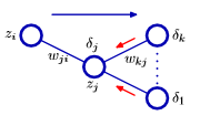
\[\delta_j = h'(a_j)\sum_k w_{kj}\delta_k\]That is, $\delta_j$ for a hidden unit can be obtained by using the $\delta$’s of the neurons in the following layer (figure from Bishop).
From here, with all the $\delta$s computed, we can use whichever update rule we wish in order to update the corresponding weights $w$.