The minimum description length principle is an approach for the model selection problem. It is underpinned by the beautifully simple concept of learning as compression. Any pattern or regularity in the data can be exploited to compress the data. Hence we can equate the two concepts - the more we can compress, the more we know about the data!
Before we begin, I would like to give thanks to Peter D. Grünwald and his text, The Minimum Description Length Principle, whose first chapter serves as the basis for this post.
1. Learning as Compression
Consider the following sequences as datasets $D$:
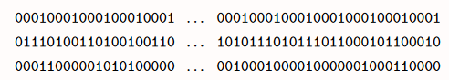
The first sequence is just a repetition of $0001$ - clearly extremely regular. The second is randomly generated, with no regularity. The third contains 4 times more 0s than 1s, and is a middle ground - less regular than the first, but more regular than the second.
To formalize the concept of MDL, we will need a description method which maps descriptions to datasets and vice-versa. One example is a computer language, where a corresponding description would then be a program that outputs the dataset $D$.
The first sequence, for example, can be easily expressed as a loop printing $0001$, which can be shown is a compression on the order of $O(\log n)$ bits. On the other hand, with a high probability, the shortest program that can output sequence 2 will be a print statement. Due to its random nature, the sequence cannot be compressed at all. The third sequence can be shown to be compressible to $O(n)$.
If we continue with computer languages as our description method, the minimum description length will be given by the length of the shortest program that can output the sequence and halt. This is the Kolmogorov complexity of the sequence. One might think that this would vary based on the hcoice of language, but according to the invariance theorem, for long enough sequences $D$, the lengths of the shortest programs in different languages will differ by a constant factor independent of $D$.
However, this idealized MDL we have arrived at using computer languages is not computable. It can be shown that no program exists that can take $D$ and return the shortest program that outputs $D$.
We are thus forced to use a more practical version of MDL, where we rely on more restrictive description methods, denoted $C$. We need to be able to compute the minimum description length of data $D$ when using said description method $C$.
2. Model Selection
To further motivate our study of MDL, consider the following example of choosing a polynomial fit, again courtesy of Grünwald:
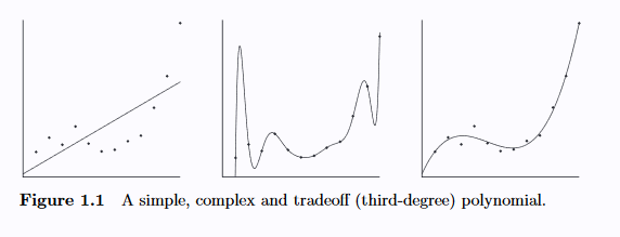
The first polynomial, which is linear, seems to suffer from high bias. It is overly simplistic. On the other hand, the second polynomial seems to suffer high variance - it is overly complex and has likely fit to the noise in the data. The third appears to generalize the best between bias and variance. MDL will provide a way to make this decision, without handwavy arguments.
Let a hypothesis refer to a single probability distribution or function, and a model refer to a family of probability distributions/functions with the same form. For example, in a polynomial fitting problem, hypothesis selection is the problem of selecting the degree of a polynomial and the corresponding parameters, whereas model selection is strictly choosing the degree.
2.1 Crude MDL
Crudely: Let $M^1, M^2, …$ be a set of candidate models. The best hypothesis $H \in M^1\cup M^2\cup …$ to compress data $D$ minimizes:
\[L(H) + L(D|H)\]$L(H)$ is the length in bits of the description of $H$ $L(D|H)$ is the length in bits of the description of $D$ encoded using $H$
Then the best model is the smallest model containing $H$.
For probabilistic hypotheses, a straightforward choice for the description method is given by $L(D|H)=-\log{P(D|H)}$, the Shannon-Fano code. Finding a code for $L(H)$, however, is hard, because the description length of a hypothesis $H$ can be very large in one model but short in another.
2.2 Refined MDL
In what is known as refined MDL, developed by Rissanen et al. (1996), we will use a one-part code $\bar L(D|M)$ instead of the two-part $L(H) + L(D|H)$. This will allow us to avoid the problem of specifying $L(H)$.
The stochastic complexity of the data given the model is given by
\[\bar{L}(D|M)\]Where by definition, this quantity will be small whenever there is some hypothesis $H \in M$ such that $L(D|H)$ is small.
$\bar{L}(D|M)$ - the stochastic complexity of the data given the model
This can itself be decomposed into:
\[\bar{L}(D|M) = L(D\|\hat{H}) + COMP(M)\]where $\hat{H}$ is the best hypothesis in $M$ (the distribution that maximizes the probability of the given data $D$), and $COMP(M)$ the parametric complexity of the model $M$. The parametric complexity measures the model’s ability to fit random data - an idea of its richness, or complexity. Recall that we are minimizing $\bar{L}(D|M)$ - we avoid overfitting by penalizing overly complex models thru the parametric complexity term.
3. The MDL Philosophy
According to Grünwald, MDL informs a “radical” philosophy for statistical learning and inference, with the following main points:
- Regularity as compression - the goal for statistical inference is compression. It is to distill regularity from noise. Refer to the example in section 1.
- Models as languages - models are interpretable as languages for describing properties of the data. Individual hypotheses capture and summarize different patterns in the data. Notice that these patterns exist and are meaningful whether or not $\hat H \in M$ is the true distribution of $D$.
- We have only the data - In fact, the concepts of “truth” and “noise” lose meaning in the MDL approach. Traditionally we assume some model generates the data and that noise is a random variable relative to this model. But in MDL noise is not a random variable. The “noise” is relative to the choice of model $M$ as the residual number of bits used to encode the data once $M$ is specified! Under the MDL principle, “noisy data” is just data that could theoretically be easily compressed using another model. This avoids what Rissanen describes as a fundamental flaw in other statistical methods, which assume the existence of a “ground truth” lying within our chosen model $M$. For instance, linear regression assumes Gaussian noise; Gaussian mixture models assume the data is generated from underlying Gaussian distributions. These are not true in practice! MDL, in contrast, has an interpretation that relies on no assumptions but the data.
4. MDL in Regression
Consider a regression setting. To describe the description length of our model $\hat y$ and the data, we code two things - the residual $r = y - \hat{y}$, and the model (the parameters). In regression, this will be encoding 1. the features that are present in the model, and 2. the associated weights.
The idea is that the residual term will be proportional to the test error, and the remaining term (the model parameters) will describe the model complexity, such that minimizing the sum (the minimum description length) minimizes the expected test error.
4.1 Residuals
First we code the residual. The optimal coding length is given by entropy - we can look at the entropy of $r$ in terms of the log-likelihood of $y$:
\[-\log{P(D|w,\sigma)} = -n\log{(\frac{1}{\sigma\sqrt{2\pi}})} + \frac{1}{2\sigma^2}\sum_i(y_i-w^Tx_i)^2\] \[-\log{P(D|w,\sigma)} = n\log{(\sigma\sqrt{2\pi})} + \frac{Err}{2\sigma^2}\]The second term is the scaled sum of squares error. The problem is we don’t know $\sigma^2$.
If we knew the true $w$, then for the corresponding $\hat{y}$, $\sigma^2=E((y-\hat{y})^2)=\frac{Err}{n}$ by the definition of variance. We don’t know it, but we can use our estimate of it.
Using our estimate at the current iteration, we get $\frac{Err^t}{2Err^t/n}=\frac{n}{2}$, which is not helpful - it’s constant. But here we refer back to the likelihood’s constant term $n\log{(\sigma\sqrt{2\pi})}$, which remains.
\[n\log{(\sigma\sqrt{2\pi})} = n\log{(\sigma)} + ...\]Where … is some term which we can safely ignore, since it is independent of $\sigma$. We know:
\[n\log{(\sigma)} \sim n\log{\sqrt{\frac{Err}{n}}} = \frac{n}{2}\log{\frac{Err}{n}}\]So ultimately we have
\[-\log{P(D|w,\sigma)} \sim \frac{n}{2}\log{\frac{Err}{n}} \sim n\log{\frac{Err}{n}}\]4.2 Weights
We can code the model by asking: for each feature, is it in the model? and if so, what is its coefficient?
Say we have $p$ features and we expect $q$ to be in the model. Then the probability is $\frac{q}{p}$. The entropy is:
\[-\sum_i \frac{q}{p}\log{(\frac{q}{p})} + \frac{p-q}{p}\log{(\frac{p-q}{p})}\]Two special cases that will come in handy below:
- If $q=\frac{p}{2}$, the cost of coding each feature presence or absence is 1 bit.
- If $q=1$ then $\log{(\frac{p-q}{p})} \sim 0$ and the cost of coding each feature is $\sim -\log{(\frac{1}{p})} = \log{(p)}$ bits
To code the weight values, this is handwavy - but the variance of $\hat{w} \sim \frac{1}{n}$, hence we use $\log{\sqrt{n}} = \frac{\log{(n)}}{2}$ bits for each feature.
So ultimately the description length is:
\[n\log{\frac{Err}{n}} + \lambda|w|_0\]Where
\[\lambda=\log{(\pi)} + \frac{\log{(n)}}{2}\] \[\pi=\frac{q}{p}\]4.3 Limiting Cases
Recall our discussion of MDL as training error + parametric complexity. Clearly the first term is capturing training error (the residuals) and the second the parametric complexity. Consider some limiting cases for $\lambda$:
- BIC - $\sqrt{n} >\hbox{}> p$ - the cost of coding feature presence is negligible; we essentially charge $\frac{\log{(n)}}{2}$ per feature.
- RIC - $p >\hbox{}> \sqrt{n}$ - the cost of coding weights is negligible; we essentially charge $\log{(p)}$ bits per feature
- AIC - $q \sim \frac{p}{2}$ and $n, p$ small - we charge 1 bit per feature.
Depending on $n, p$ and our expected $q$ a different penalty criterion $\lambda$ is more appropriate to describe the variance.