Here I’ll briefly introduce the idea of kernels, a powerful mathematical concept that allows us to easily incorporate nonlinearity in models.
1. Kernels
Suppose we have a mapping $\phi : \mathbb{R}^n \rightarrow \mathbb{R}^m$ taking our vectors $x$ in $n$ space to $m$ space. The dot product of $x, y$ in this space is $\phi(x)^T\phi(y)$.
The kernel is a function $k$ corresponding to this dot product:
\[k(x, y) = \phi(x)^T\phi(y)\]The Gram matrix is a matrix $G$ with elements $G_{i,j} = k(x_i, x_j) = \phi(x_i)^T\phi(x_j)$. A function $k$ is a valid kernel iff the Gram matrix is positive semi-definite (symmetric, and all eigenvalues are $\geq 0$).
The value of the kernel is in the technique of kernel substitution, or the kernel trick. We can compute $\phi(x)^T\phi(y)$ by first mapping the data using the feature transformation $\phi$, then taking the dot product. Or, if we know the kernel function, we can simply use that without ever explicitly using or knowing $\phi$ at all!
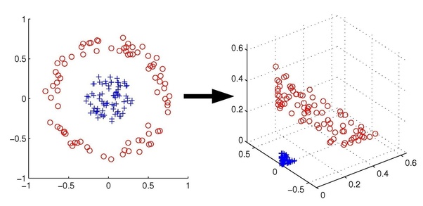
Many thanks to Prof. Jordan and UC Berkeley for the image and the following example.
In this example image, our data is not linearly separable in $\mathbb{R}^2$. However, if we map it to $\mathbb{R}^3$, it is!
As an aside - we have taken our linear SVM algorithm and applied it to our transformed data, and gotten a nonlinear algorithm for free! This is the power of kernels.
Back to the kernel trick. Here this feature mapping is:
\[(x_1, x_2) \rightarrow (z_1, z_2, z_3) = (x_1^2, \sqrt{2}x_1x_2, x_2^2)\]We could calculate $\langle\phi(x_i),\phi(x_j)\rangle$ by taking $x_i, x_j$ into feature space first:
\[\langle\phi(x_i),\phi(x_j)\rangle = \langle(x_{i1}, x_{i2}),(x_{j1}, x_{j2})\rangle\] \[\langle\phi(x_i),\phi(x_j)\rangle = \langle(x_{i1}^2, \sqrt{2}x_{i1}x_{i2}, x_{i2}^2),(x_{j1}^2, \sqrt{2}x_{j1}x_{j2}, x_{j2}^2)\rangle\] \[\langle\phi(x_i),\phi(x_j)\rangle = x_{i1}^2x_{j1}^2 + 2x_{i1}x_{i2}x_{j1}x_{j2} + x_{i2}^2x_{j2}^2\]Or, if we knew the kernel function corresponding to this feature mapping $\phi$, which is $k(x_i, x_j) = \langle x_i, x_j \rangle^2$, we could have done this:
\[\langle\phi(x_i),\phi(x_j)\rangle = \langle(x_{i1}, x_{i2}),(x_{j1}, x_{j2})\rangle\] \[\langle\phi(x_i),\phi(x_j)\rangle = (x_{i1}x_{j1} + x_{i2}x_{j2})^2\] \[\langle\phi(x_i),\phi(x_j)\rangle = x_{i1}^2x_{j1}^2 + 2x_{i1}x_{i2}x_{j1}x_{j2} + x_{i2}^2x_{j2}^2\]Which is much less computationally expensive! If we know the kernel function we don’t even need $\phi$ explicitly at all!
One great example is in the SVM formulation. We can replace $\phi(x_n)\phi(x_m)$ with kernel functions, allowing us to easily apply the classifier to any arbitrary feature space!
2. Linear regression example
Another example is the classic linear regression. Using the concept of duality, we can reformulate the loss function in terms of inner products $\phi(x_i)^T\phi(x_j)$ and hence in terms of kernel functions.
2.1 Setup
Consider minimizing the regularized sum of squares error function, given $N$ observations of data $x$:
\[J(w) = \frac{1}{2}\sum_{n=1}^N(w^T\phi(x_n)-y_n)^2 + \frac{\lambda}{2}w^Tw\]Setting $\frac{\partial J}{\partial w}=0$, the solution for $w$ is a linear combination of the $\phi(x_n)$:
\[w=\frac{-1}{\lambda}\sum_{n=1}^N(w^T\phi(x_n)-y_n)\phi(x_n)\] \[w=\sum_{n=1}^Na_n\phi(x_n)\] \[w=\Phi^Ta\]where $\Phi$, the design matrix, has rows given by $\phi(x_n)^T$ and $a=(a_1, …, a_N)^T$, where $a_n = \frac{-1}{\lambda}(w^T\phi(x_n)-y_n)$
2.2 Dual representation
We can reformulate this problem in terms of $a$ instead of $w$. Substitute $w$ back into $J(w)$:
\[J(a) = \frac{1}{2}a^T\Phi\Phi^T\Phi\Phi^Ta-a^T\Phi\Phi^Ty+\frac{1}{2}y^Ty+\frac{\lambda}{2}a^T\Phi\Phi^Ta\]where $y=(y_1, …, y_n)^T$
Define the Gram matrix $K=\Phi\Phi^T$, with $K_{nm}=\phi(x_n)^T\phi(x_m)=k(x_n, x_m)$
We can solve for $a$ by plugging $w=\Phi^Ta$ into the definition of $a$:
\[a=(K+\lambda I_N)^{-1}y\]Substitute this back in the model. For a new input $x^*$:
\[\hat{y}(x^*) = w^T\phi(x^*) = k(x^*)^T(K+\lambda I)^{-1}y\]where $k_n(x) = k(x_n, x^*)$
The value is that we have expressed the solution to the least squares problem entirely in terms of the kernel function $k(x, x’)$!
Recall the MLE solution $w=(X^TX)^{-1}X^Ty$. That is, we had to invert a $M\times M$ matrix ($m$ here is the number of features - the number of columns). To get $a$ we need to invert $K + \lambda I$ which is $N\times N$. This is typically not good - usually $N \gg M$. However, because the dual formulation is expressed entirely in terms of the kernel function, we can avoid having to explicitly calculate this inverse!
Another common application of kernels is in kernel density estimation, which will come in another post.