It always helps to have an intuition for the geometric meaning of a model. This is typically emphasized in the case of common models such as linear regression, but there are relatively few discussions of this for logistic regression. It is especially interesting in this case to draw the distinction between logistic regression and support vector machines.
In classification, we want to find a decision boundary in feature space that separates our classes. Specifically in logistic regression, which is a linear classifier, we are simply looking for a decision hyperplane.
But how do we choose the separating hyperplane? Even in the simplest case of a linearly separable dataset, there are many candidates. Suppose we have two points in $\mathbb{R}^2$.
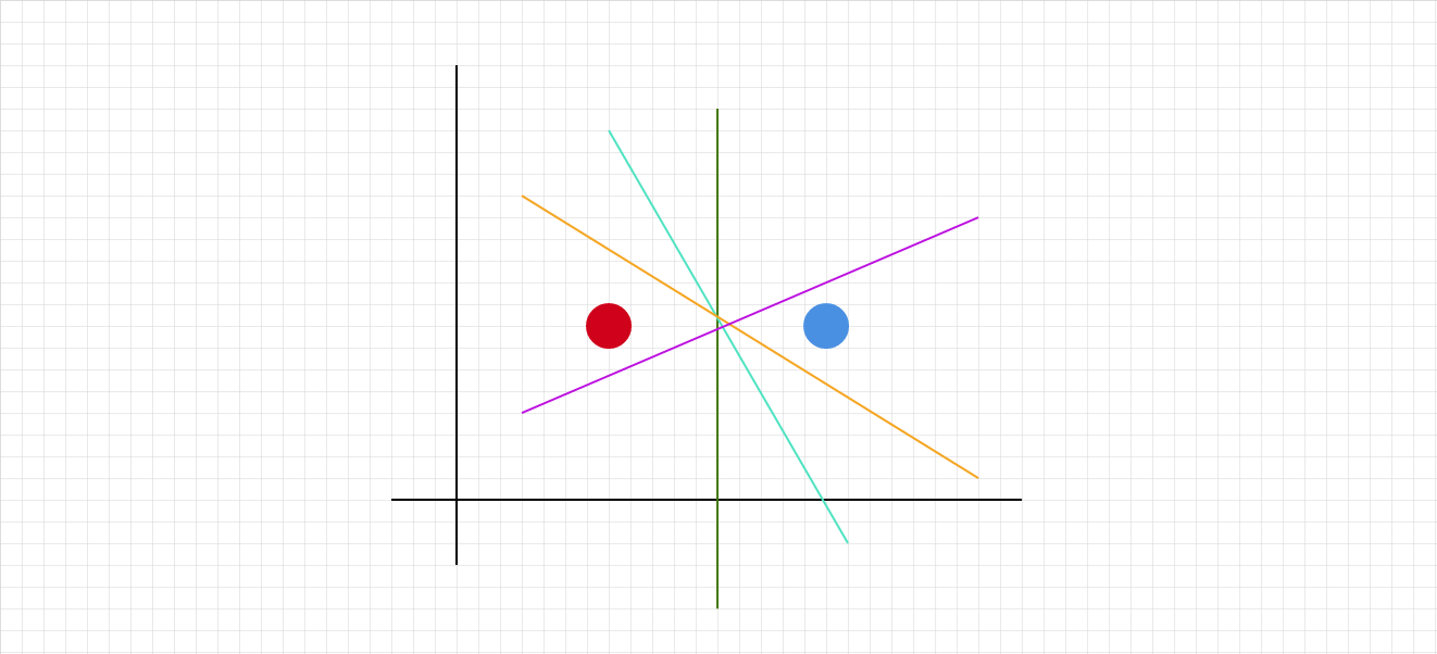
All of these colored lines are separating decision lines! Which one will logistic regression select?
1. Logistic regression refresher
Recall in (binary) logistic regression we are modeling the conditional class probabilities:
\[P(C_1|x, w)=\sigma(w^Tx)\]That is, given the data $x$ and the learned weights $w$, what is the probability of class $C_1$?
Further recall that $a = w^Tx$ where
\[a = \log{\frac{p(x|C_1)p(C_1)}{p(x|C_2)p(C_2)}}\] \[a = \log{\frac{p(C_1|x)}{p(C_2|x)}}\]It represents the log of the odds ratio. There are three cases:
\[\frac{p(C_1|x)}{p(C_2|x)} = 1, p(C_1|x) = p(C_2|x), a = 0\] \[\frac{p(C_1|x)}{p(C_2|x)} > 1, p(C_1|x) > p(C_2|x), a > 0\] \[\frac{p(C_1|x)}{p(C_2|x)} < 1, p(C_1|x) > p(C_2|x), a < 0\]Let $y \in \{-1, 1\}$ denote the two classes. Then,
\[P(y_i=1|x_i, w) = \sigma(w^Tx)\]It follows that
\[P(y_i=-1|x_i, w) = 1-\sigma(w^Tx) = \sigma(-w^Tx)\]The final step comes from the properties of the sigmoid function:
\[\sigma(-x) = 1-\sigma(x)\]It is easy to verify - remember that $\sigma(x) = \frac{1}{1+\exp(-x)}$.
Notice that these expressions can be consolidated:
\[P(y=y_i|x_i, w) = \sigma(y_iw^Tx_i)\]2. Projections refresher
Projecting a vector $b$ onto a subspace $A$ is simply picking out the part of $b$ that lies in $A$. Take the simplest example, in $\mathbb{R}^2$, of projecting a line $b$ onto another line $A$. The projection $p$ is the part of $b$ along $A$.
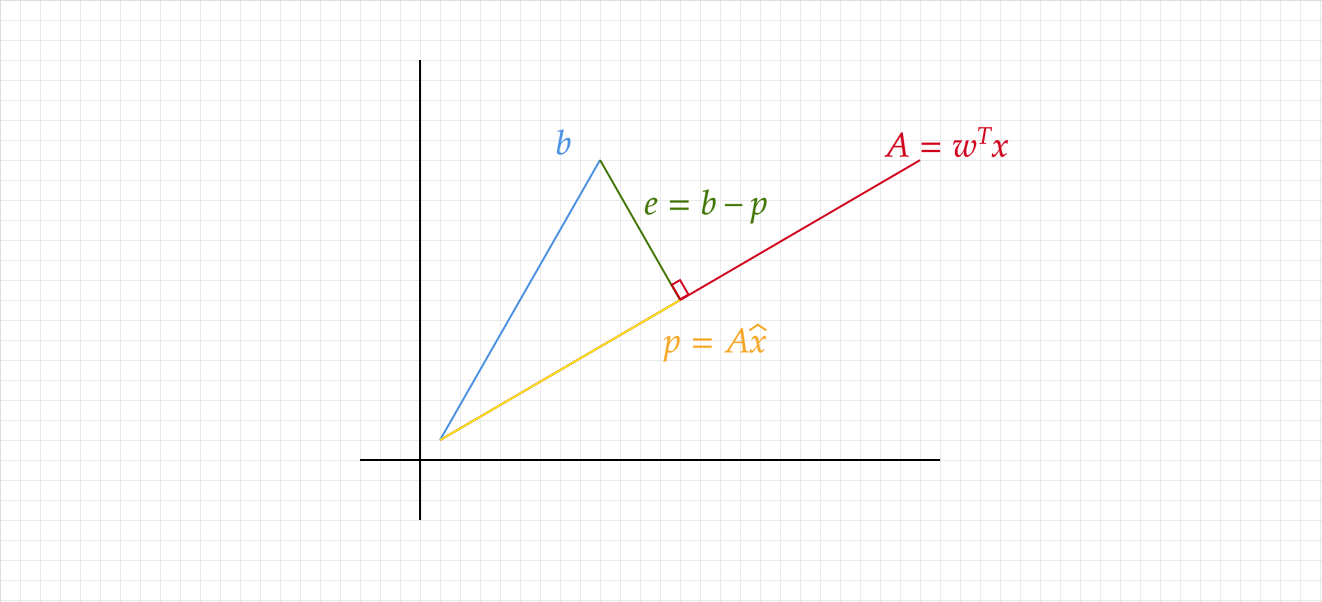
Notice that $p$ is some multiple $\hat{x}$ of $A$ by definition, so $p = A\hat{x}$. Let $e = b - p$ be the error, or the vector from $b$ to the closest point on $A$. Critically, $e \perp A$! By this orthogonality:
\[A \cdot e = 0\] \[A \cdot (b - e) = 0\] \[A \cdot (b - A\hat{x}) = 0\] \[\hat{x} = \frac{A^T}{A^TA}b\] \[p = A\hat{x} = \frac{AA^T}{A^TA}b\]I took some liberties with the notation - recall that $A\cdot b$ is equivalent to $A^Tb$.
3. The geometry
Armed with the above, we are prepared to discuss the geometry.
\[P(y=y_i|x_i, w) = \sigma(y_iw^Tx_i)\]There are two key points:
First, consider the quantity $y_iw^Tx_i = y_ia_i$, the margin of classification. Using what we deduced above, $y_i, a_i$ will have the same sign iff the model correctly classified the class of observation $x_i$. And if it is negative, then the training label $y_i$ and the model disagree.
Second, remember that $w^Tx = w_1x_1 + w_2x_2 + … = 0$ is the definition of a hyperplane. It represents, in fact, the separating decision hyperplane we discussed in the beginning. What is the distance $d$ to the plane $w^Tx = 0$ of a point with vector $x_i$?
Remember from the definition of a plane that the normal vector to the plane $w^Tx = 0$ is given by $w$. Let $X$ be some point on the plane $w^Tx = 0$. We can arrive at $d$ by projecting $x_i-X$ onto $w$, and making use of the fact that $w^TX = 0$.
\[d = ||\text{proj}_w(x_i-X)||\] \[d = ||w\frac{w^T(x_i-X)}{w^Tw}||\] \[d = ||w\frac{w^Tx_i-w^TX}{w^Tw}||\] \[d = ||w\frac{w^Tx_i}{w^Tw}||\] \[d = ||\frac{w^Tx_i}{w}||\] \[d = \frac{|w^Tx_i|}{||w||}\]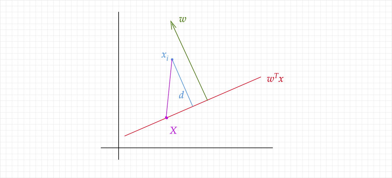
The classification margin $y_iw^Tx_i$ is proportional to the distance $d$ to the hyperplane $w^Tx$. It quantifies the model’s confidence in its classification of $x_i$. This matches up with the meaning of $w^Tx_i = a_i$, the log odds ratio! And the sigmoid function simply normalizes things by squashing everything into the $[0, 1]$ range - into a probability.
Now recall the likelihood function we want to maximize in logistic regression:
\[P(y|X, w) = \prod_i P(y=y_i|x_i, w) = \prod_i \sigma(y_iw^Tx_i)\]The sigmoid applied to a large, negative margin will be close to $0$. A small negative margin, approaching $0.5$. A large positive margin, approaching $1$. So to maximize the likelihood, we want the classification margins for each training example to be large, positive values - confident and correct classifications!
Ultimately, we are finding a separating hyperplane that is maximizing the product of the sigmoid-transformed classification margins, over ALL points in the training set.