Ensemble methods express the simple and effective idea of strength in numbers. They combine multiple models together in order to improve performance over a single model in isolation. Here we will discuss some common methods in use today.
1. Bagging
A simple method to start with is bootstrap aggregating, or bagging. The idea is basic - we will just average our predictions over several individual models. The trick is that we have only one training set to do this with - how can we introduce variance among our individual models?
1.1 Bootstrapping
Recall how bootstrapping works. We sample $N$ points from our training set with replacement - some data points can be duplicated in each bootstrap sample - to generate a “new” dataset. We are sampling from our training set just like how the training set is randomly sampled from the original population! By bootstrapping we obtain an idea about the variability within our data.
For example, suppose we want to estimate the average weight of people in the US. It is not feasible to weigh everyone - instead we take a random sample of $N$ people and measure their weights. From this sample we arrive at merely one estimate of the average weight. But if we take $M$ bootstrap samples from our dataset and calculate the average weight in all of those samples, we now have $M$ bootstrap estimates of the average, giving us an idea of the distribution of the sample mean. Of course, we can generalize this methodology to other statistics and estimators, not just means, as we shall see below.
1.2 Applying bootstrapping to a regression estimator
Suppose we are in a regression setting. Denote the data $x$, a model for this training data of the form $y(x)$, and the true underlying function $h(x)$.
Generate $M$ bootstrap samples and train estimators $y_m(x)$ on each sample. Then our overall prediction is just the average over all $M$:
\[y_{bag}(x) = \frac{1}{M}\sum_{m=1}^My_m(x)\]That’s all there is to bagging algorithmically, but we can go further and prove some properties of bagging and investigate why it helps.
We will express the mean-squared error of the models $y_m(x)$ individually, then compare that to the mean-squared error of $y_{bag}(x)$.
1.2.1 Individual errors
Notice that we can write:
\[y_m(x) = h(x) + \epsilon_m(x)\]That is, the output of each bootstrap estimator is the true value plus some noise denoted by $\epsilon$.
Then the expected value of the mean-squared error, with respect to the distribution of $x$, is:
\[E_x((y_m(x)-h(x))^2) = E(\epsilon_m(x)^2)\]So the average error of the models $y_m(x)$ can be written:
\[E_1 = \frac{1}{M}E_x(\sum_{m=1}^M\epsilon(x)^2)\]1.2.2 Aggregated error
Now, the expected value of the error after bagging is:
\[E_m = E_x((\frac{1}{M}\sum_{m=1}^My_m(x) - h(x))^2)\] \[E_m = E_x((\frac{1}{M}\sum_{m=1}^M\epsilon_m(x))^2)\] \[E_m = \frac{1}{M^2}E_x(\sum_{m=1}^M\epsilon_m(x)^2 + \sum_{m\neq l}^M\epsilon_m(x)\epsilon_l(x))\]If we can assume that the errors $\epsilon_m(x)$ are unbiased (zero mean) and uncorrelated:
\[E_x(\epsilon_m(x)) = 0\] \[E_x(\epsilon_m(x)\epsilon_l(x)) = 0\]then we can cancel the second term to obtain:
\[E_m = \frac{1}{M^2}E_x(\sum_{m=1}^M\epsilon_m(x)^2)\]Notice that this is:
\[E_m = \frac{1}{M}E_1\]We have reduced the average error of the model by a factor of $M$ by simple averaging!
However, this result is dependent on the faulty assumption that the errors are uncorrelated - in reality they are usually highly correlated. Nevertheless, this gives some intuition for a reduction in error via bagging.
1.3 Bias-variance tradeoff
Bagging reduces the variance of our model. Intuitively, by averaging over the results over $M$ bootstrap samples, their individual errors cancel each other out when we combine results into the final $y_{bag}(x)$.
1.4 Out-of-bag error
Notice that the probability of not having a particular observation in a bootstrap sample is $(1-\frac{1}{n})^n$, which converges to $\frac{1}{e} \approx 37\%$. That is, for each bootstrap sample, $\approx 37\%$ of observations are excluded, forming what we call an “out-of-bag” set.
For each bootstrap sample, the error estimation can simply be done on this out-of-bag set! By averaging these errors over all bootstrap samples we obtain an out-of-bag estimate of prediction error - all without cross-validation or a holdout set.
1.5 Random Forests
Random forests are a combination of bagging and decision trees. Decision trees are a great base estimator for bagging - they are prone to high variance and overfitting, since they can always achieve zero training error.
We simply generate $M$ bootstrap samples and build decision trees on each sample, then aggregate the results at the end. We can use a mean for regression outputs and majority voting in classification tasks.
2. Boosting
Boosting is another ensembling method aggregating several models together.
2.1 AdaBoost
We start with the widely used AdaBoost (adaptive boosting) algorithm. While it can be adapted for regression, in the interest of keeping things simple I’ll stick to classification.
Whereas in bagging we simply averaged over the predictions of base models trained on bootstrap samples, in boosting we will train base models sequentially over iteratively weighted forms of the dataset. Observations that are misclassified by a base classifier will be given greater weight in the dataset passed on to the next classifier to be trained. By continuously reweighting the dataset, we are saying that certain examples are more important to classify correctly than others.
Finally we will combine all the base classifiers $y_1(x), …, y_M(x)$ using weighted voting:
\[y(x) = sign(\sum_{m=1}^M\alpha_my_m(x))\]AdaBoost works as follows:
We are given $N$ observations $(x_i, t_i)$ where $t_i \in \{(-1, 1\}$.
- Initialize weights $w_n^{(1)} = \frac{1}{N}$ for each observation
- For $m = 1:M$
- Fit classifier $y_m(x)$ by minimizing the weighted error function:
- Calculate:
which is a weighted error rate of the $m$th classifier on the dataset. We can use it to calculate the classifier weights:
\[\alpha_m = \ln{\frac{1-\epsilon_m}{\epsilon_m}}\]which are the log-odds of the classifier being correct on the weighted dataset. The following plot helps visualize:
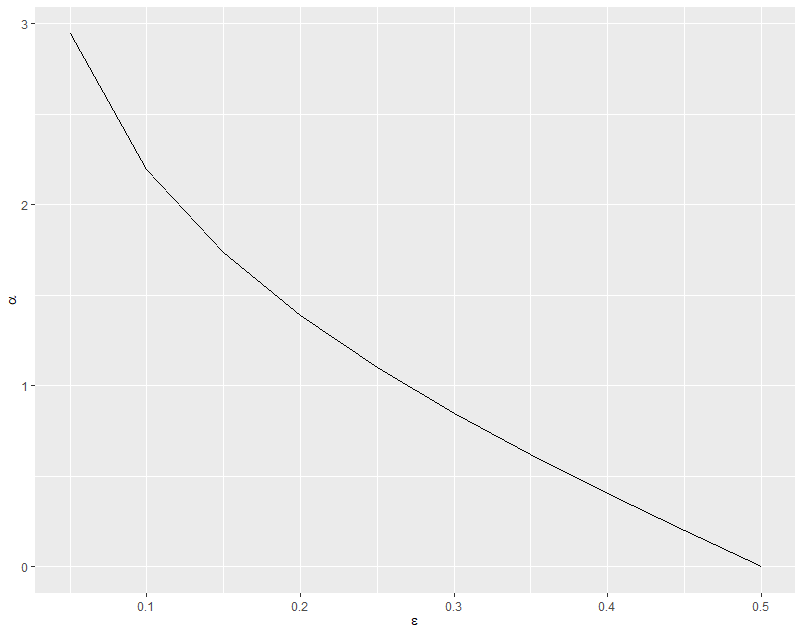
So for lower weighted error rate $\epsilon$ we have a larger classifier weight $\alpha$.
- Update the data weights
- Make the final prediction
The first classifier has weights $w_n^{(1)}$ that are uniform. It is business as usual for training the classifier. But in subsequent iterations the weights increase for points that are incorrectly classified (the indicator function will be 1) and do not change for points that are correctly classified (the indicator function is 0).
2.1.1 AdaBoost as minimizing exponential error
AdaBoost can be explained as sequential minimization of an exponential loss, which can be shown through the following derivation. Let’s define:
\[f_m(x) = \frac{1}{2}\sum_{l=1}^m\alpha_ly_l(x)\]which is a classifier formed by a weighted sum of the base classifiers $y_l(x)$. Then the prediction $y(x)$ is just $sign(f_m(x))$.
Define the exponential error function:
\[E = \sum_{n=1}^N\exp{(-t_nf_m(x_n))}\]We want to minimize this training error w.r.t the weights $\alpha$ as well as the parameters of the base classifiers. But instead of doing this globally, we do it sequentially, i.e. the base classifiers $y_1(x), …, y_{m-1}(x)$ and their coefficients $\alpha_1, …, \alpha_{m-1}$ are fixed. Rewrite the error function:
\[E = \sum_{n=1}^N\exp{-t_nf_{m-1}(x_n) - \frac{1}{2}(-t_n\alpha_my_m(x_n)}\] \[E = \sum_{n=1}^Nw_n^{(m)}\exp{(-\frac{1}{2}t_n\alpha_my_m(x_n))}\]where
\[w_n^{(m)} = \exp{(-t_nf_{m-1}(x_n))}\]since only $y_m(x), \alpha_m$ are not fixed. Now we can reformulate this:
\[E = e^{-\alpha_m/2}\sum_{n\in A_m} w_n^{(m)} + e^{\alpha_m/2}\sum_{n\in B_m} w_n^{m}\]where $A_m, B_m$ are the set of points classified correctly and incorrectly by our classifier $y_m(x)$, respectively. This then becomes:
\[E = (e^{\alpha_m/2} - e^{-\alpha_m/2})\sum_{n=1}^Mw_n^{(m)}I(y_m(x_n)\neq t_n) + e^{-\alpha_m/2}\sum_{n=1}^Mw_n^{(m)}\]When we minimize by taking the partial w.r.t $y_m(x)$, we will recover the AdaBoost weighted error function:
\[J_m = \sum_{n=1}^Nw_n^{(m)} I(y_m(x_n)\neq t_n)\]And when we take the partial w.r.t $\alpha_m$ we will recover:
\[\alpha_m = \ln{\frac{1-\epsilon_m}{\epsilon_m}}\]For the data weights, first notice:
\[w_n^{(m+1)} = \exp{(-t_nf_{m}(x_n))}\] \[w_n^{(m+1)} = \exp{(-t_n(\frac{1}{2}\sum_{l=1}^m\alpha_ly_l(x)))}\] \[w_n^{(m+1)} = \exp{(-t_n\alpha_my_m(x_n)(\frac{1}{2}\sum_{l=1}^{m-1}\alpha_ly_l(x_n)))}\] \[w_n^{(m+1)} = w_n^{(m)}\exp{(-t_n\alpha_my_m(x_n))}\]Take a moment to convince yourself that this is true:
\[t_ny_m(x_n) = 1 - 2I(y_m(x_n) \neq t_n)\]And plug that into the above to arrive at:
\[w_n^{(m+1)} = w_n^{(m)}\exp(-\frac{\alpha_m}{2})\exp{(\alpha_mI(y_m(x_n) \neq t_n)}\]Since $\exp(-\frac{\alpha_m}{2})$ is independent of $n$, it is uniform across all $n$ observations, so we are free to drop it. So we have finally arrived at our AdaBoost update equation:
\[w_n^{(m+1)} = w_n^{(m)}\exp{(\alpha_mI(y_m(x_n)\neq t_n))}\]2.1.2 AdaBoost vs. logistic regression
Recall the logistic regression likelihood function:
\[P(y|X, w) = \prod_i P(y=y_i|x_i, w) = \prod_i \sigma(y_iw^Tx_i)\]Maximizing this is equivalent to minimizing
\[\sum_i\log(1+\exp{(-y_iw^Tx_i)})\]which is just taking the log likelihood and flipping the fraction of the sigmoid to turn the maximization problem into a minimization.
So we are minimizing $\log(1+\exp(-y_iw^Tx_i))$
Boosting is effectively minimizing $\exp(-y_i\alpha^T(x_i))$
Below is a plot of these loss functions, along with the hinge loss in SVM.
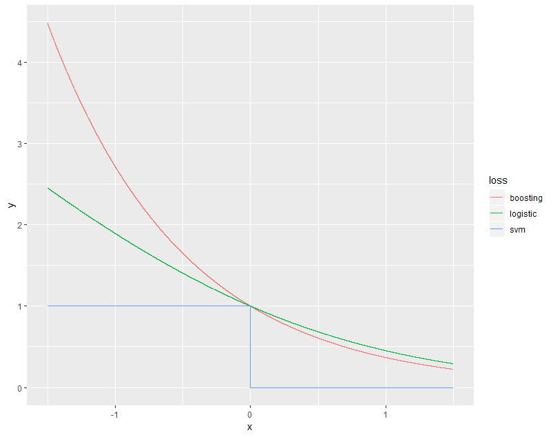
Notice that the exponential loss is more sensitive to misclassification - it penalizes examples on the wrong side of the decision boundary at an exponential rate, vs. the linear growth of the cross-entropy. Of course SVM, in stark contrast to the others, only cares about whether an example is on the correct side or not - nothing more.
The exponential loss also cannot be interpreted as nicely as the cross-entropy, as the log-likelihood of a probabilistic model. So we lose that interpretability.
Furthermore, cross-entropy is generalizable to multiclass problems, whereas exponential loss cannot.
2.2 Gradient boosting
Now let’s briefly discuss gradient boosting in relation to our above derivations for AdaBoost.
We showed above how AdaBoost is just sequential optimization of an additive model with exponential loss. This is an important perspective to have, because it also shows that we can extend boosting to regression problems by changing the exponential loss to something more appropriate like sum-of-squares error.
However, minimizing arbitrary loss functions, even when we’re doing them sequentially in the boosting paradigm, can be computationally infeasible. In gradient boosting, we tackle this thru approximation - we iterate on $f_m(x)$ by taking a step in the direction of the minimum gradient w.r.t $f_{m-1}(x)$. We avoid overfitting by fitting our successive learners $y_m(x)$ to the gradient of the loss function w.r.t $f_{m-1}(x)$.
So AdaBoost is a special case with a specific exponential loss function, which allows it to be interpreted as iterative reweighting on the dataset to emphasize misclassified observations. Gradient boosting, on the other hand, is a more generic approach to the additive modeling problem posed in boosting.